Introduction to HPC, shared memory parallel using openmp

1 The multicore system

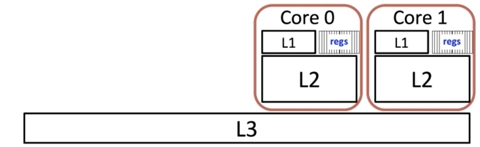
The relationship with L1-L3 cache. The L3 cache is shared, but every core have its own L1-2 cache.

2 Using openmp

1

#include "omp.h"

Before using it, we need to define how many threads we want to use:

In Unix system:

1

export OMP_NUM_THREADS=4 

The instruction:

1

#pragma omp parallel

If we put this macro before one line of code or one block, the line or block will be executed $OMP_NUM_TRHREADS times.

The instruction:

1

#pragma omp parallel for

will seperate the for loops into different pieces for threading.

3 optimization of threading

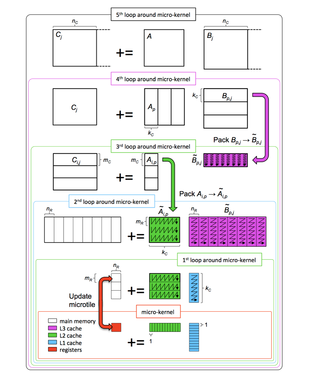
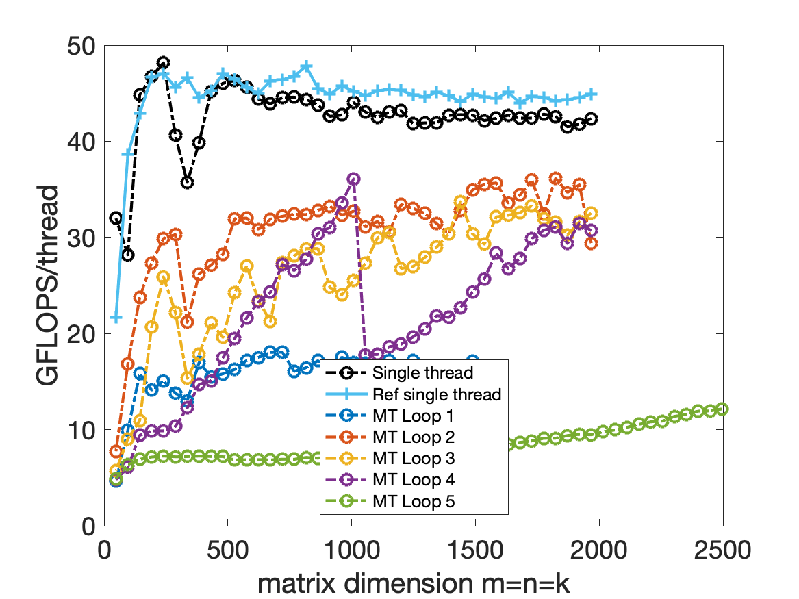
Consider the previous five for-loop, we could use #pragma omp parallel for before one of the for loop. And this is the results of the performance, note the y-axis is GFLOPS/thread.

Analysis

In MT Loop1, the performance is not good because every core L2 cache must load the submatrix of A. And in this sample, the Mc = 72, Mr=8, that means in every 1st for loop, only $\frac{Mc}{Mr} = 9$ tasks need to be executed by 4 threads, the ratio of tasks over threads is too small. This will cause the imbalance of load. Besides the amortized expense is very large.(Computer system need to do branching and synchronization operation, this will also need time to execute.)

In MT Loop2, the performance is good. The only downside is every core need to store the same $A_{i,p}$ matrix in L2 cache.

In MT Loop3, it is a little tricky. Because only add the parallel instruction, you will not get the right answer. That is because in the code we only have a buffer for Atilde(the packing matrix), but all threads will write to A simutaneously, and the Atilde will not be correct for every one threads. Lucky thing is that if the size of this loop (m/Mc) is not large, we could apply for extra matrix, and every thread will have its own Atilde.

 1
 2
 3
 4
 5
 6
 7
 8
 9
10
11
12
13
14

// Code loop 3
void LoopThree( int m, int n, int k, double *A, int ldA, double *Btilde, double *C, int ldC )
{
  double *Atilde = ( double * ) _mm_malloc( MC * KC * omp_get_max_threads() * sizeof( double ), 64 );
       
  #pragma omp parallel for
  for ( int i=0; i<m; i+=MC ) {
    int ib = min( MC, m-i );    /* Last loop may not involve a full block */
    PackBlockA_MCxKC( ib, k, &alpha( i, 0 ), ldA, &Atilde[ MC * KC * omp_get_thread_num() ] );
    LoopTwo( ib, n, k, &Atilde[ MC * KC * omp_get_thread_num() ], Btilde, &gamma( i,0 ), ldC );
  }

  _mm_free( Atilde);
}

In MT Loop4, this algorithm is not correct. Because every threads will write to the matrix simutaneously. The C can’t accumulate, this will lead to the error. Of course you could make another matrix to store the value temporarily, but it is too expensive.

In MT Loop5, the performance will change with the quotient $\frac{n}{N_C}$.

4 Ahmdahl’s law

Consider a sequential algorithm that solves the problem in time $T$.

Suppose a fraction $f$ of this work cannot be parallelized, while the remaining $1-f$ scales perfectly across $t$ threads. The total time with $t$ threads becomes

$$

\begin{equation*} T_t = \frac{(1-f)T}{t} + fT = T\left(f + \frac{1-f}{t}\right) \end{equation*}

$$

and it is immediate that $T_t \geq fT$.

For matrix multiplication we can write the sequential cost as $$

\begin{equation*} T(n) = 2 n^3 \gamma + C n^2 \beta \end{equation*}

$$ so the parallel execution time is $$

\begin{equation*} T_t(n) = \frac{2 n^3 \gamma}{t} + C n^2 \beta \end{equation*}

$$ The speedup coefficient is therefore $$

\begin{equation*} S_t(n) = \frac{T(n)}{T_t(n)} = \frac{2 n^3 \gamma + C n^2 \beta}{\frac{2 n^3 \gamma}{t} + C n^2 \beta} \end{equation*}

$$ and the efficiency simplifies to $$

\begin{equation*} E_t(n) = \frac{S_t(n)}{t} = \frac{2 n^3 \gamma + C n^2 \beta}{2 n^3 \gamma + t C n^2 \beta} \end{equation*}

$$ As $n \to \infty$, the lower-order term involving $C n^2 \beta$ vanishes and $E_t(n) \to 1$: larger problem sizes deliver higher efficiency.