Hierarchy Memory
1. Why use Hierarchy Memory
Because the register memory is much faster than main memory, in fact the difference is about two magnitude. And the performance gap will be larger because the CPU’s speed increase faster than main memory.
In this situation, if we fetch data from the main memory too many times, the expense will be very expensive. But if we create some memory which is faster than main memory but a little bit slower than register memory. We call it cache.
The cache memory is bigger than register memory, if every time we fetch data from main memory to cache firstly, then the register will extract data and return result to cache, which is faster. After all data completed, the register will communicate with main memory and get another batch of data.
Usually the expense of fetching data from register memory to cache is cheap. And because cache is larger so every time we could fetch more data from main memory. This means we could decrease the frequency of fetching data. Which will save a lot of time.

2. Cache algorithm
In order to make the algorithm easy to analyse, we assume that the main memory will exchange data with cache and cache will exchange with register.
In order to simiplify this model, we assume in the data exchange procedure, there is no calculation(in fact they can do simultaneously, just image that the main memory update while cache change data with register, it is easy to achieve.)

This inspire us, that if the matrix size is smaller, which is smaller than L1-L3 cache size, the data will be all stored in cache, and it is very fast. So we make an algorithm:
We divide the matrix as many micro-tile:

Note that:


This algorithm means that we can use micro kernel algorithm to realize the operation in the three-for-loop: $$ \begin{equation*} C_{i, j}:= A_{i, p} B_{p, j}+C_{i, j} \end{equation*} $$
The block matrix $C_{i,j}$ ,$A_{i,p}$ and $B_{p,j}$ small block matrix, which are submatrix. We define the ijp loop as level 1 for loop. The algorithm to realize
$$ \begin{equation*} C_{i, j}:= A_{i, p} B_{p, j}+C_{i, j} \end{equation*} $$
as level 2 loop.
Terminology
A $m_R\times n_R$ submatrix of C is called micro-tile
The $m_R\times k_C$ , $k_C\times n_R$is called micro-panles
The routine that updates a micro-tile by multiplying two micro-panels we will call the micro-kernel.
Review the picture:
If we want to maintain good performance, the size of the micro-tile algorithm can be equal to L2 cache.
And according to the estimate, the best size of the three matrix can be:
96x96. (Because the L2 cache is 256KBytes, we want to find the matrix size which is the multiple of 12(because 12 is multiple of 2 4 6 12), then 96 is the most suitable)
The algorithm can be show using this picture:

Then we use the algorithm, the micro-kernel algorithm can use 4x4 or 12x4, compare their performance:

The size of micro-kernel should consider the size of L1 cache and register.
2.1 Test for different outer for loop

From the result above we can see that the micro-kernel is not sensitive to the outer for loop. But the size of micro Kernel will related to the speed of MMM.
3.2 performance analysis
In the micro kernel for loop, we use vector intrinsic function:
Assume we have the square matrix, and their sizes are the same:
So the b is larger, more time you will use in computation rather than transferring data.
- note that the data transferring expense in cache to main memory is more than 100 times than floats operation.
- In practice the movement of the data can often be overlapped with computation (this is known as prefetching). However, clearly only so much can be overlapped, so it is still important to make the ratio favorable.
3.3 Algorithm improvments
- Streaming submatrix of B and C.
Consider previous algorithm:

Every time we put 3 submatrix into the cache, but according to the calculation, the larger of the submatrix, the better performance. Note that every time in fact we do streaming operation, just use a little piece of A and a panel of B.
So we can do this instead:

Every time we put the colored space into L2 cache, that means we could store larger submatrix of A(the blue part) to get better efficiency. And every time, we pick up micro panel of A and streaming micro panel of B and streaming micro-tile of C to finish calculation.
$m_c$,$n_c$ and $k_c$ are dimensional of submatrix of C, A and B.
If we use a 4x4 micro kernel algorithm, then we can continue divide the submatrix into micro kernel and using streaming method:
$m_r\times 4= m_c$, $n_r\times 4= n_c$, $k_r\times 4= k_c$

In the L2 cache, use JIP for rank-1 operation for calculating submatrix multiplication. J is the outer for loop, then in this processdure we can keep the matrix of A stay in L2 cache, stay for the all loop, then every time we just need to stream the micro kernel of submatrix C and B(in the picture is the red and green part).
The algorithm above is just an example, of course you could make the whole submatrix of B in the L2 cache, just change the order of the micro-kernel loop is OK.
A smarter method.
In the previous part, we use PIJ loop to take apart the A, B and C matrix. In this method, we will load the same $A_{i,p}$ submatrix for many times. We could do better to optimize this, and we could compress the PIJ for loop to PI for loop. This will decrease the number which the same block of A will loaded.
The picture will show the procedure:

That means every time we move the submatrix of A($m_c\times k_c$) into the L2 cache , and stream the red and green part from main memory to L2 cache.
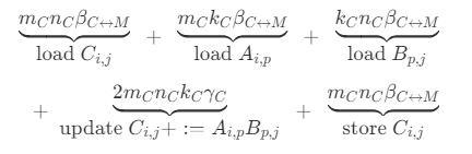
Each Level 2 for loop’s expense is:
$$ \begin{equation*} \begin{array}{rcl} \begin{array}{c} \underbrace{ m_C n \beta_{C \leftrightarrow M}} \ \text{load}~C_{i,j} \end{array} + \begin{array}{c} \underbrace{ m_C k_C \beta_{C \leftrightarrow M}} \ \text{load}~A_{i,p} \end{array} + \begin{array}{c} \underbrace{ k_C n \beta_{C \leftrightarrow M}} \ \text{load}~B_{p,j} \end{array} \[0.2in] + \begin{array}{c} \underbrace{ 2 m_C n k_C \gamma_C} \ \text{update}~C_{i} +:= A_{i,p} B_{p} \end{array} + \begin{array}{c} \underbrace{ m_C n \beta_{C \leftrightarrow M}} \ \text{store}~C_{i,j} \end{array} \end{array} \end{equation*} $$ And the summary is: $$ \begin{equation*} \begin{array}{c} \underbrace{ m_C k_C + \left( 2 m_C n + k_C n \right) \beta_{C \leftrightarrow M} } \ \text{data movement overhead} \end{array} + \begin{array}{c} \underbrace{ 2 m_C n k_C \gamma_C } \ \text{useful computation} \end{array} \end{equation*} $$
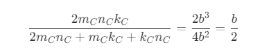
The ratio of use ful computation and data movement expense is:
$$ \begin{equation*} \frac{ 2 m_C n k_C} { 2 m_C n + m_C k_C + k_C n }. = \frac{2 b^2 n}{3b n + b^2} \approx \frac{2 b^2n}{3bn} \approx \frac{2b}{3} \end{equation*} $$
is a little better than PIJ level 1 For loop’s performance.
This is the comparison of PIJ v.s. PI Level 1 For loop:

No large difference, I use the newest software, may be the compiler have automatic optimization function for this problem.
3.4 Find the best $A_{i,p}$ size
Using the last streaming algorithm, we can calculate all possible situation to get the best performance size of micro tile: $m_C\times k_C$
After trying different size of the submatrix of A.

From this figure, we can see that the best size of the submatirx of A is 192x40.
Performance Analysis
For this procedure, the analysis method is to calculate the ratio of computation and memory operation.

Every time we store the blue part of A for multiple usage, and streaming the submatrix of B and C, that means the marked part in the picture. We should compute the how many effective computation after we read from A, B and C. For submatrix of A, it could be reused for many streaming operation of B and C, thus the analysis base is not the same.
Bring an $mC \times kC$ submatrix of A into the cache, at a cost of $m_C \times k_C\beta_{M \leftrightarrow C}$, And the floats is:$2m_Ck_Cn$, the ratio is, $$ \frac{floats}{memory\ operation}=\frac{2n}{\beta_{M\leftrightarrow C}} $$ The larger n, the better ratio(performance).
This analysis didn’t consider the streaming cost of submatrix of C and B.
For the micro-kernel operation:
Every time we read a submatrix of B: $$ \frac{floats}{memory\ operations} = \frac{2m_C}{\beta’_{M\leftrightarrow C}} $$
For the micro-kernel operation:
Every time we read a submatrix of C: $$ \frac{floats}{memory\ operations} = \frac{2m_Ck_Cn_R}{2m_Cn_R\beta’’{M\leftrightarrow C}}=\frac{k_C}{\beta’’{M\leftrightarrow C}} $$
We should make sure the $m_C$, $k_C$ as large as enough.
3.5 Blocking for L1 and L2 cache
If we want to do better, we could use L1 and L2 cache properly. The micro-tile is small could be use in register memory. Then keep submatrix of A in L2 cache and streaming micro-panel of B to L1 cache, which is faster.
This algorithm’s Level 1 for loop is the same as 3.4, the smarter method, which is show in the picture at the main memory part.

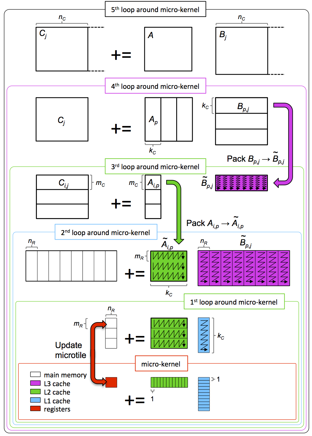
3.6 Blocking for L1 L2 and L3 cache

The for loop procedue can be illustrated using this picture:

Every for loop, we can know from the picture what the loop do in this level. and the code is attached:
| |
And this is the performance of the implementation:

which is much better. And 12x4 micro-kernel is very good.
4 Packing in MMM
4.1 Stride matters
From the picture:
We can see that the performance will go down with the matrix dimension. When the size is small, its efficiency is good, but when the size become larger, it will tends to a lower constant.
In our experiment, if we at first will create a matrix of leading dimension is 1500x1500, and use submatrix to do the experimental ,like the picture :
we will get the result(Five_Loops_12x4Kernel_Ldim).
That is because the data is not continous, which is not packed tightly. So it will decrease the efficiency of the algorithm.
The result also related to some conceptiong about memory pages(4kb) and cache prefetching technique.
Memory page:
https://en.wikipedia.org/wiki/Page_(computer_memory).Cache prefetching:
https://en.wikipedia.org/wiki/Cache_prefetching.
Note that the prefetching only allow for the size continuously below 4kb, so once the matrix become larger, the prefetching will not be executed. Thus the performance goes down.
Note
The packing operation will need some extra operation, but if we amortize the expense, the performance will still increase.
4.2 Packing of A and B
In order to let the matrix become continuous memory we should pack the submatrix of A and B.
Apply for a extra memory to store packed submatrix of B (the Btilde):
The code is:
| |
We divide submatrix of B into many micro-panels and packed them separately. But the Btilde is continous on Kc x Nc.
Then packing A and store Atilde into L2 cache:

| |
We also divide this as many micro-panels to packed them separately:
| |
The packing procedure can also been showed in five-loop procedure:
Note that in each micro panel, the memory is continous, and for submatrix of B, the counting method is not column-major, it is row-major. When we do rank-1 operation in micro-kernel procedure, the memory of A and B are continuous.

(The memory is continous because of the packing or renumbering)
We can see that now the performance of Five_Loops_Packed_12x4Kernel perform very closed to the reference.
In the small matrix size, the performance is not good that because the computation expense is much smaller than data transferring expense. The amortized cost of coping a matrix is very high.
Then in the end find the optimal Mc and Kc:

5. Recommandation for HPC
Using vector intrinsic.
Avoid repeatting transfer data.
Block the MMM to make good use of cache.
Broadcasting A and loading elements of B.(not so effective)
It sounds very complicated, but there is a smart way to realize this:
By defining( this means these matrice are row-major):
1
2
3
#define alpha( j,i ) A[ (j)*ldA + i ] #define beta( j,i ) B[ (j)*ldB + i ] #define gamma( j,i ) C[ (j)*ldC + i ]Loop unrolling.
This will decrease the time for branching prediction.

(with 12x4 and 4x4 loop unrolling)
We can see nothing changed, the improvement of 12x4 and 4x4 is not so obvious.
https://zh.wikipedia.org/wiki/分支預測器
https://zh.wikipedia.org/wiki/循环展开
Prefetching (tricky; seems to confuse the compiler…)
Using in-lined assembly code
useful link:https://github.com/flame/blis/blob/master/kernels/haswell/3/old/bli_gemm_haswell_asm_d6x8.c
Note:
https://github.com/flame/blis/blob/master/kernels/haswell/3/old/bli_gemm_haswell_asm_d6x8.c